Valentine’s Day Spending
Examining the Data
<- readr:: read_csv ("https://raw.githubusercontent.com/rfordatascience/tidytuesday/master/data/2024/2024-02-13/gifts_age.csv" )
Rows: 6 Columns: 9
── Column specification ────────────────────────────────────────────────────────
Delimiter: ","
chr (1): Age
dbl (8): SpendingCelebrating, Candy, Flowers, Jewelry, GreetingCards, Evenin...

ℹ Use `spec()` to retrieve the full column specification for this data.
ℹ Specify the column types or set `show_col_types = FALSE` to quiet this message.
Rows: 6
Columns: 9
$ Age                 <chr> "18-24", "25-34", "35-44", "45-54", "55-64", "65+"
$ SpendingCelebrating <dbl> 51, 40, 31, 19, 18, 13
$ Candy               <dbl> 70, 62, 58, 60, 50, 42
$ Flowers             <dbl> 50, 44, 41, 37, 32, 25
$ Jewelry             <dbl> 33, 34, 29, 20, 13, 8
$ GreetingCards       <dbl> 33, 33, 42, 42, 43, 44
$ EveningOut          <dbl> 41, 37, 30, 31, 29, 24
$ Clothing            <dbl> 33, 27, 26, 20, 19, 12
$ GiftCards           <dbl> 23, 19, 22, 23, 20, 20
categorical variables:
  name     class levels n missing                                  distribution
1  Age character      6 6       0 18-24 (16.7%), 25-34 (16.7%) ...

quantitative variables:
                 name   class min    Q1 median    Q3 max     mean        sd n
1 SpendingCelebrating numeric  13 18.25   25.0 37.75  51 28.66667 14.733183 6
2               Candy numeric  42 52.00   59.0 61.50  70 57.00000  9.777525 6
3             Flowers numeric  25 33.25   39.0 43.25  50 38.16667  8.886319 6
4             Jewelry numeric   8 14.75   24.5 32.00  34 22.83333 10.870449 6
5       GreetingCards numeric  33 35.25   42.0 42.75  44 39.50000  5.089204 6
6          EveningOut numeric  24 29.25   30.5 35.50  41 32.00000  6.066300 6
7            Clothing numeric  12 19.25   23.0 26.75  33 22.83333  7.359801 6
8           GiftCards numeric  19 20.00   21.0 22.75  23 21.16667  1.722401 6
  missing
1       0
2       0
3       0
4       0
5       0
6       0
7       0
8       0
Data Munging & Creating Data Dictionary
<- gifts_age %>% mutate (Age = as.factor (Age))
# A tibble: 6 × 9
  Age   SpendingCelebrating Candy Flowers Jewelry GreetingCards EveningOut
  <fct>               <dbl> <dbl>   <dbl>   <dbl>         <dbl>      <dbl>
1 18-24                  51    70      50      33            33         41
2 25-34                  40    62      44      34            33         37
3 35-44                  31    58      41      29            42         30
4 45-54                  19    60      37      20            42         31
5 55-64                  18    50      32      13            43         29
6 65+                    13    42      25       8            44         24
# ℹ 2 more variables: Clothing <dbl>, GiftCards <dbl>
Age
Factor-qual
Age group
SpendingCelebrating
Float-quant
Average spending on celebrations
Candy
Float-quant
Average spending on candy
Flowers
Float-quant
Average spending on flowers
Jewelry
Float-quant
Average spending on jewelry
GreetingCards
Float-quant
Average spending on greeting cards
EveningOut
Float-quant
Average spending on evening outings
Clothing
Float-quant
Average spending on clothing
GiftCards
Float-quant
Average spending on gift cards
Research Questions
Dependent variable- spending
Independent variable - age
-Relation between age and gift categories
-what are the valentine’s day spending trends across different age groups
What research activity might have been carried out to obtain the data graphed here?
plotting graph
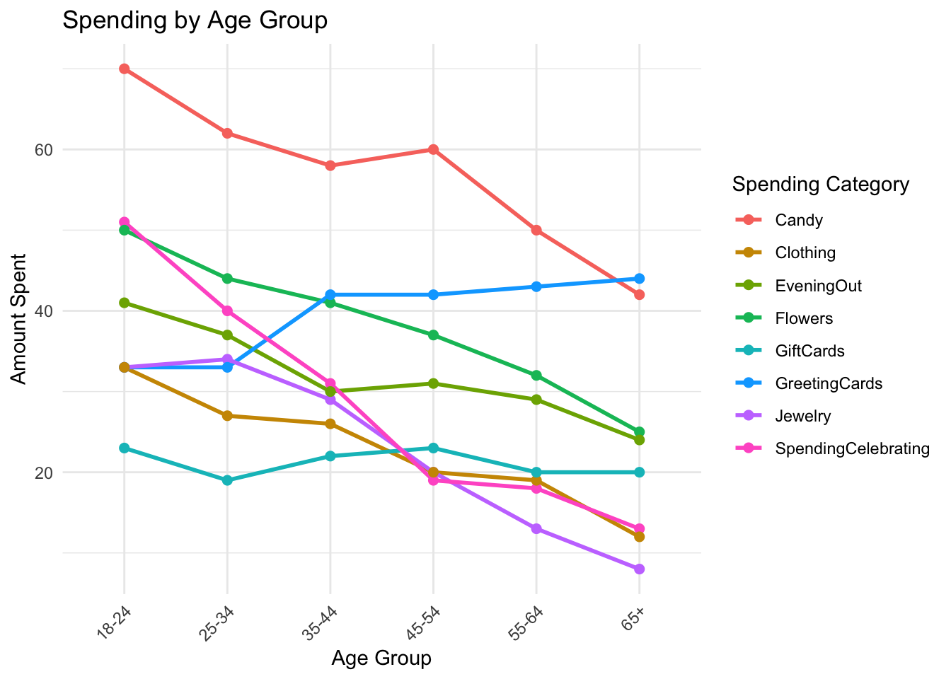
<- gifts_age %>% pivot_longer (cols = - Age, names_to = "Category" , values_to = "AmountSpent" ) ggplot (data_long, aes (x = Age, y = AmountSpent, color = Category, group = Category)) + geom_line (size = 1 ) + geom_point (size = 2 ) + labs (title = "Spending by Age Group" ,x = "Age Group" ,y = "Amount Spent" ,color = "Spending Category" ) + theme_minimal () + theme (axis.text.x = element_text (angle = 45 , hjust = 1 ))
Warning: Using `size` aesthetic for lines was deprecated in ggplot2 3.4.0.
ℹ Please use `linewidth` instead.
Pre processing: wide to long where all spending categories are combined in one column which becomes our amount spent.
colnames (giftsage_modified)
[1] "Age"                 "SpendingCelebrating" "Candy"
[4] "Flowers"             "Jewelry"             "GreetingCards"
[7] "EveningOut"          "Clothing"            "GiftCards"
[1] "Age"                 "SpendingCelebrating" "Candy"
[4] "Flowers"             "Jewelry"             "GreetingCards"
[7] "EveningOut"          "Clothing"            "GiftCards"
Observations/surprises
-Did not expect spending on jewellery to be high among the younger age brackets.
- had a preconceived notion that the 65+ age group would have considerable amounts of spending in the jewellery and flowers categories
-did not expect candy to be plotted so high up either especially for the older age groups.